R.version.string2 Getting Started with R
The above is called a yaml (or yml) header. It provides the script with instructions it will execute when we save our document at the end of the session.
Introduction
- This guide shows how to:
- Video 1
- Download and install R and RStudio
- Understand how base R differs from RStudio
- Choose a CRAN mirror
- Navigate the RStudio environment (the 4 panes)
- Format flat files (like CSV) for loading
- Create objects
- Install and load libraries
- Format files for loading
- Load a dataset (flat file and pointers to other resources)
- Video 2
- Run simple calculations
- Learn the types of objects
- Create functions
- Create snippets
- Conduct basic analyses
- Save datasets
- Save and render Quarto files
- Learn where to find help
- Sources for further reading
2.0.1 VIDEO 1
2.1 Download This Lesson and Run It Locally
If you want your own copy of this Quarto file:
- Open
R_basics.qmdin this GitHub repository. - Click Raw and save the file, or use Code > Download ZIP for the full repository.
- Open the file in RStudio.
- Run code chunks with
Cmd/Ctrl + Enter, or render from a terminal:
quarto render R_basics.qmd --executeSee the full setup and troubleshooting steps in Run R Basics Locally.
3 The R Project Homepage
The official home of the R language is The R Project for Statistical Computing:
- Website: https://www.r-project.org/ (copy/paste the link without the < > to open it now)
From this site you can access:
- Links to CRAN (the Comprehensive R Archive Network) for downloads
- Manuals, FAQs, and contributed documentation
- Source code and news about new versions of R
This site is the “home base” for R itself and is separate from RStudio/Posit (which provides the Integrated Development Environment (IDE)).
4 How to Download R and RStudio, and Check Your Versions
4.1 Installing R and RStudio
- R is the programming language and engine.
- RStudio (by Posit) is a popular Integrated Development Environment (IDE) for R.
An IDE is a software environment that integrates coding, running, and debugging tools in one place, making programming easier and more efficient.
Install R first, then RStudio.
- Download R (CRAN; The Comprehensive R Archive Network)
- Go to https://cran.r-project.org/
- Click “Download R for Windows”, “macOS”, or “Linux”
- Choose the latest release and run the installer
- Go to https://cran.r-project.org/
- Download RStudio Desktop (free)
- Go to https://posit.co/download/rstudio-desktop/
- Download the installer for your operating system and run it
- Open RStudio after installing (R should already be installed)
- Go to https://posit.co/download/rstudio-desktop/
4.2 Checking Your Versions
4.2.1 R version
4.2.2 RStudio version
# If running inside RStudio, this will show RStudio version:

if (exists("RStudio.Version"))
  paste("RStudio version:", RStudio.Version()$version)
Explanation:
RStudio.Version is a function provided by RStudio. If it is run inside RStudio, it returns a list of metadata, including “version”. We are calling only for the version using the $ operator.
paste simply fronts the version with “RStudio version” so that it prints nicely.
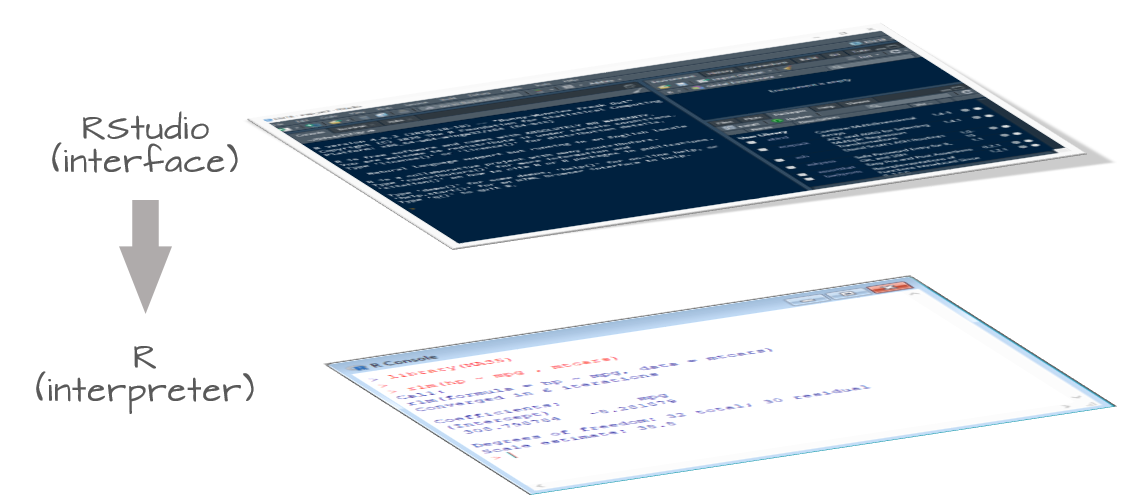
5 How Base R Differs from RStudio
- Base R
- The language + interpreter/engine
- Comes with a console and basic GUI (varies by OS)
- You can run scripts and commands via the R console or terminal
- RStudio IDE (by Posit)
- A graphical environment wrapping R
- Offers script editor, plotting viewer, environment browser, package manager, project management, and integrated help
- Makes development, reproducibility, and visualization easier, but does not replace R itself
Example: Base R functionality (works the same in RStudio since RStudio calls R under the hood)
6 What Is a CRAN Mirror and How Do You Set It?
CRAN (The Comprehensive R Archive Network) hosts R itself and thousands of R packages.
Because CRAN is mirrored (copied) around the world, you typically choose a CRAN mirror close to you geographically so downloads are faster and more reliable.
You can set your CRAN mirror interactively:
# This opens a menu in R to choose a CRAN mirror:
# chooseCRANmirror()   # uncomment and run once in a session

# I am in Seattle as I record this, so I chose #68, as OHSU is the CRAN mirror that is geographically closest to me.
Or you can set it programmatically in your script:
# Example: set CRAN mirror via options() for this session (you only need to run one of these, and only run it once)
# options(repos = c(CRAN = "https://ftp.osuosl.org/pub/cran/"))
# options(repos = c(CRAN = "https://cloud.r-project.org"))

# or this CRAN mirror (uncomment, if needed to run)
# options(repos = c(CRAN = "https://cran.r-project.org"))
6.1 You can check current repos with:
getOption("repos")7 Setting a Working Directory and Using R Projects
R needs to know where your files live. This is your working directory.
A very efficient workflow is to:
- Create a work folder for your project.
- Create an R Project inside that folder.
- Keep all your data, code, and documents in that folder.
7.1 Creating an .Rproj and Setting the Working Directory
Create a .Rproj file, name it, and save it in your new work folder:
- File → New Project → Existing Directory (or “New Directory” to create a new folder)
To create and save your R Script file:
- File → New File → Quarto Document…
- File → Save (choose
.Rextension)
- For R Markdown: File → New File → R Markdown, then Save as
.Rmd
Once you are in your R Project, the working directory will automatically be the project folder.
Check your working directory:
getwd()You can change the working directory manually (less recommended than using Projects):
# Example only; adjust to your own path:
# setwd("/path/to/your/project/folder")
Using R Projects is more robust than calling setwd() in every script, and it keeps your projects self-contained.
8 Exploring the RStudio Environment (Panes and Toolbars)
Once you have installed R and RStudio, open RStudio. By default, you will see four main panes:
- Source (top-left)
- Your editor for
.Rscripts,.Rmd,.qmdfiles
- Run code lines or chunks into the Console
- Your editor for
- Console (bottom-left)
- Where R commands execute
- Shows outputs, errors, warnings
- Where R commands execute
- Environment/History (top-right)
- Environment: data frames and objects currently in memory
- History: previously run commands
- Environment: data frames and objects currently in memory
- Files/Plots/Packages/Help/Viewer (bottom-right)
- Files: browse project files
- Plots: view figures
- Packages: installed packages and load/unload controls
- Help: documentation for functions and packages
- Viewer: renders HTML content (e.g., Quarto documents)
- Files: browse project files
Across the top toolbar you will find buttons for:
- Running code chunks or single lines
- Knitting (for
.Rmd) or Rendering (for.qmd)
- Managing Projects and version control (Git)
- Creating new scripts and Quarto / R Markdown files
- Saving files
This Quarto figure syntax that embeds an image and centers it using a figure attribute block. 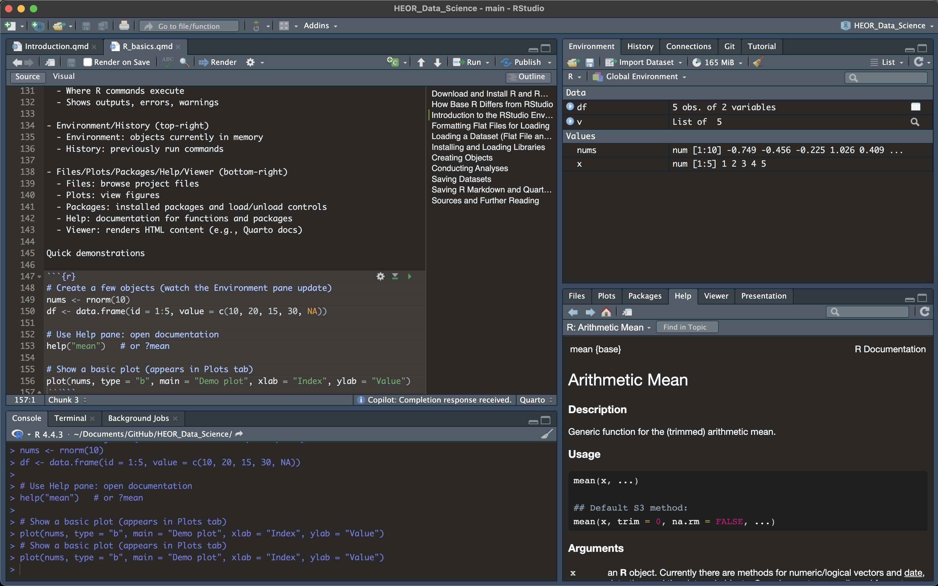
9 Now you are ready to get started!
Create a code chunk by typing 3 backticks and then {r}. End the code chunk by typing 3 more backticks. Naming each chunk helps to debug when knitting/rendering (see below).
# I type my code here (without the hash). It is easiest to debug if you separate it into chunks like this. # To run the code you have 3 options:
# (1) highlight the line and press Run (in the upper right),
# (2) place your cursor at the end of the line and type Cmd/Ctrl + Enter, or
# (3) to run the entire chunk, click on the green button to the right. 9.1 Quick Demonstrations
# Create a few objects (watch the Environment pane update)
nums <- rnorm(10)
df <- data.frame(id = 1:5, value = c(10, 20, 15, 30, NA))

# Use Help pane: open documentation
help("mean")   # or ?mean
This is code that will insert an image when we render the document.
# Show a basic plot (appears in Plots tab or below)
plot(nums, type = "b", main = "Demo plot", xlab = "Index", ylab = "Value")
# b is commanding R to create both points and lines.
10 Installing and Loading Libraries
R’s functionality is extended through packages (libraries). You typically:
- Install a package once (per machine or environment).
- Load it in each session where you want to use it.
10.1 Installing Packages
10.1.1 Install a single package
# Example install - (run once; set eval: false to avoid automatic install).
# or install pacakges from within the Console.

install.packages("dplyr")
install.packages("ggplot2")
10.1.2 Install multiple packages at once
# Example install of multiple packages (run once; set eval: false to avoid automatic install).
# or install packages from within the Console.

install.packages(c("readr", "readxl", "data.table"))
10.2 Loading Packages
10.2.1 Load a single package
# Load dplyr package
library(dplyr)
10.2.2 Load multiple packages safely
# Load if available; fall back gracefully if not
loaded_pkgs <- c()
for (pkg in c("dplyr", "ggplot2")) {
  if (requireNamespace(pkg, quietly = TRUE)) {
    library(pkg, character.only = TRUE)
    loaded_pkgs <- c(loaded_pkgs, pkg)
  }
}

# This code creates an empty vector to track successfully loaded packages.
# loops through the list of package names.
# checks whether each package is installed.
# loads the package if it is installed.
# tells library that the variable contains the package name as text.
# records the packages that were loaded. (if it is not installed, it isn't loaded)
loaded_pkgs
Notes:
- Use
install.packages("packagename")once per machine or project.
- Use
library(packagename)in each session/script where needed.
- For reproducibility, consider project environments such as renv.
- renv creates an isolated package library per project and:
- records the exact package versions you used
- lets others (or future-you) recreate the same setup
11 Formatting Flat Files for Loading
Good practices for CSV/TSV flat files:
- Use a header row with short, clear, alphanumeric column names
(avoid spaces; use underscores if needed)
- Use UTF-8 encoding
- Use a consistent delimiter (comma for CSV, tab for TSV)
- Represent missing values consistently (e.g., empty cell or
NA; avoid “-”, “N/A”, “null”)
- Use ISO 8601 for dates (
YYYY-MM-DD) and include time zones if timestamps are present
- Avoid embedded line breaks in cells; if present, ensure proper quoting
- Keep one “tidy” table per file: each row is one observation, each column is one variable
11.1 Create and Save a Well-Formatted CSV
# Example tidy dataset
tidy_example <- data.frame(
  subject_id = 1:6,
  group = c("control", "control", "control", "treatment", "treatment", "treatment"),
  age_years = c(34, 45, 51, 29, 40, NA),
  visit_date = as.Date(c("2025-01-10", "2025-01-12", "2025-01-13", "2025-01-11", "2025-01-12", "2025-01-14")),
  score = c(87, 90, 85, 92, 88, 91)
)

# Create a data folder, then save CSV
dir.create("data", showWarnings = FALSE)
csv_path <- file.path("data", "tidy_example.csv")
write.csv(tidy_example, csv_path, row.names = FALSE, na = "")

csv_path

# dir.create, file.path and wrte.csv are all R functions native to R.
# dir.create("data") creates a data folder in the current working directory.
# file.path builds a file path that works on any operating system.
# "data" is the folder I am creating.
# "tidy_example" is the name of my dataset.
# csv_path is the object I have created that specifies the path where data/tidy_exmple.csv will be kept.
# write.csv saves the csv in the data folder in the working directory.
# row.names = FALSE tells R to not include the row numbers in the csv.
# na = "" tells R to save empty cells as empty cells instead of as "NA".
# check it out in your data folder!
12 Loading a Dataset (Flat File and Other Resources)
12.1 Loading the CSV with Base R
# we reload the tidy_example here by creating an object (loaded_base) and reading in from the csv_path.

loaded_base <- read.csv(csv_path, stringsAsFactors = FALSE)

# we could also have loaded it by specifying the relative path like this:
# loaded_base <- read.csv("data/tidy_example.csv")

# R's default is to set strings as factors. Sometimes the type of variable is important when manipulating variables.
str(loaded_base)  # structure of the dataframe
head(loaded_base) # first six rows (by default)
12.2 Loading the CSV by creating a new object
# here is another way to handle this. Let's say instead of loading "tidy_example" in its original form I load it by creating a tidy_example object.
# then I want to add a new variable to tidy_example and resave it.
# (because we know that simply creating an object will not add the new variable to the dataframe, nor will it save it)

# Load tidy_example data back in
tidy_example <- read.csv(csv_path)

# Add a new dichotomized variable
tidy_example$score_dichot <- ifelse(tidy_example$score > 90, 1, 0)

# Save it again (overwrite the same file)
write.csv(tidy_example, csv_path, row.names = FALSE, na = "")

head(tidy_example)
12.3 Loading the CSV with readr (tidyverse)
# Install readr if needed (run once; chunk is set to eval=FALSE so it won't execute automatically)
install.packages("readr")
# If readr is available, demonstrate its use safely
if (requireNamespace("readr", quietly = TRUE)) {
loaded_readr <- readr::read_csv(csv_path, show_col_types = FALSE)
head(loaded_readr)
}
# requireNamespace checks to see if the "readr" package is installed. This is particularly useful if you are working with others and you do not want your code to automatically add a package (readr) to their machine.
# the double-colons calls the package only when needed but does not install it. 12.3.1 Handling Column Types and Missing Values Explicitly with readr
if (requireNamespace("readr", quietly = TRUE)) {
  loaded_typed <- readr::read_csv(
    csv_path,
    col_types = readr::cols(
      subject_id = readr::col_integer(),
      group = readr::col_factor(levels = c("control", "treatment")),
      age_years = readr::col_double(),
      visit_date = readr::col_date(),
      score = readr::col_double()
    ),
    show_col_types = FALSE
  )
  str(loaded_typed)
}

# If the readr package is installed, this code will read the dsv file at csv_path, explicitly define the data type of each column, store it as loaded_typed, and print its structure.
# If the readr package is installed but not loaded as a library, the 2 colons in each row will use the readr package anyway, use to execute that row.
12.3.2 Reading Excel Files
# set eval=FALSE to prevent automatic installation.
# or install packages from within the Console.

install.packages("readxl")  # run once

if (requireNamespace("readxl", quietly = TRUE)) {
  # Example: readxl::read_excel("data/example.xlsx", sheet = 1)
}

# (We won’t read here unless a file exists)
# note that I can load just one tab of my excel workbook (sheet 1)
# if I comment out the Example line, there is nothing inside the brackets, so R will return a NULL.
12.3.3 VIDEO 2
13 Simple Calculations
# Base R calculations
x <- c(1, 2, 3, 4, 5)
# x is the object I have created. Note the object now appears in the Environment pane.
# <- is called the assignment operator.
# c starts a vector of numbers.
mean(x)
sd(x)
sum(x^2)
# I call for the mean, sd, and sum of the squared numbers in my vector.
14 Types of Objects and Variables in R
R works with several fundamental object types:
- Scalars: single values (e.g.,
x <- 5)
- Vectors: ordered collections of values of the same type
- Matrices: 2D arrays (rows × columns) of a single type
- Arrays: multi-dimensional generalization of matrices
- Data frames: tabular structures (columns can have different types)
- Lists: ordered collections of elements that can each be a different type or structure
14.1 Creating Objects in Practice
14.1.1 Scalars
scalar_example <- 42

scalar_example
14.1.2 Numeric and character vectors (scalars are simply vectors of length 1)
a <- c(10, 20, 30)

b <- c("alpha", "beta", "gamma")

a

b
14.1.3 Factors
treatment <- c("control", "treatment", "control", "treatment", "treatment", "control")

treatment

grp <- factor(treatment, levels = c("control", "treatment"))

grp
14.1.4 Matrices
# Matrices - have 2 dimensions; rows and columns
m <- matrix(1:9, nrow = 3)

m
14.1.5 Arrays
# Arrays (3-dimensional example)
arr <- array(1:24, dim = c(3, 4, 2))

arr
14.1.6 Data frames
# Data frames (tabular)
df2 <- data.frame(id = 1:6, group = grp, score = c(88, 92, 85, 91, 87, 90))

df2
14.1.7 Lists
# Lists
lst <- list(scalar = scalar_example, vector = a, matrix = m, array = arr, dataframe = df2)

lst
14.2 How Data Frames Differ from Datasets (Stata/SAS)
If you have used Stata or SAS, you may be used to “datasets” as files on disk.
In R:
- A data frame is an in-memory object, not a file.
- You typically read a file (CSV, Stata, SAS, Excel) into a data frame, work with it, then write it back out.
- R data frames are flexible: columns can have different types.
Conceptually, think of “dataset on disk” (Stata/SAS) versus “data frame in memory” (R), even though they represent similar rectangular data.
15 Coding in Base R vs RStudio
- Base R
- The language + interpreter/engine.
- Can be used from a terminal or the R GUI.
- The language + interpreter/engine.
- RStudio
- An IDE that wraps around R.
- Provides a script editor, console, plots, help, history, projects, Git integration, and more.
- An IDE that wraps around R.
You can write exactly the same R code in both environments; RStudio simply makes development more convenient.
16 R Is Open Source – Anyone Can Create an R Function
R is an open-source language, which means:
- The source code is publicly available.
- Anyone can write and share R functions and packages.
- Most R packages are maintained by individuals or teams and distributed through CRAN, Bioconductor, GitHub, or other platforms.
You can define your own functions easily:
# A simple custom function
add_two <- function(x) {
  x + 2
}

add_two(5)
# add_two is the name of the function (or the object);
# <- is the assignment operator
# function tells R you are defining a function;
# x is the input argument; # when you call add_two(5) you are saying that x takes the value of 5.
# The code inside {} is the body of the function. This is what runs when the function is called.
# x + 2 is what R will return.

# Another example: compute a z-score
z_score <- function(x) {
  (x - mean(x, na.rm = TRUE)) / sd(x, na.rm = TRUE)
}

z_score(c(1, 2, 3, 4, 5))

# x is the argument.
# mean and sd are the functions.
# 1,2,3,4,5 is the vector that comprises the dataset for the argument.
# na.rm is the option that removes missing values.
This is the same mechanism that package authors use—just organized and distributed as packages.
17 Snippets: Small Templates or Code Skeletons
Snippets are short templates of code you can insert quickly in RStudio.
Example snippet definition:
snippet fun
  ${1:fname} <- function(${2:x}) {
    ${0}
  }
colors <- function(x) {result = x + 2
return(result)
}
colors(5)To see how it works, in your R script type fun and press Tab to expand this into a function template.
To explore snippets in RStudio:
- Tools → Global Options → Code → Edit Snippets…
17.1 Create your own snippet
- Open the Snippets editor as above.
- Add a new snippet definition (e.g., for a histogram):
snippet gg_hist
    ${1:plot_name} <- ggplot(data    = ${2:data_name}, mapping = aes(x = ${3:x_var_name})) +
    geom_histogram( fill = "lightblue", color = "lightblue") +
    labs(title    = "${4:title_name}", x = "${5:x_axis_name}",y = "${6:y_axis_name}")+
theme_minimal()- Save and close the editor.
- In your script, type
gg_histand press Tab to insert the template.
18 Conducting Analyses
18.1 Descriptive Statistics (Base R)
x <- rnorm(100, mean = 50, sd = 10)
summary(x)
mean(x); median(x); sd(x); quantile(x, probs = c(0.25, 0.5, 0.75))
18.2 Group-wise Summaries (dplyr, if available)
if (requireNamespace("dplyr", quietly = TRUE)) {
  library(dplyr)
  loaded_base %>%
    group_by(group) %>%
    summarise(
      n = n(),
      mean_score = mean(score, na.rm = TRUE),
      mean_age = mean(age_years, na.rm = TRUE)
    )
}
18.3 Visualization (ggplot2, if available)
if (requireNamespace("ggplot2", quietly = TRUE)) {
  library(ggplot2)
  ggplot(loaded_base, aes(x = group, y = score, fill = group)) +
    geom_boxplot() +
    geom_jitter(width = 0.1, alpha = 0.6) +
    labs(title = "Scores by Group", x = "Group", y = "Score") +
    theme_minimal()
}

# this code says that if ggplot2 is available, please load it. If it is not available, creating the graph is optional and the code will run without it (and without creating the plot)
# ggplot requires that I must have previously created a dataframe that is in long format that it will use. In this case, loaded_base is already in the format that ggplot can use.
# ggplot has specific syntax that is easy to learn.
# here are 2 ggplot resources:
# https://www.data-to-viz.com/
# https://r-graph-gallery.com/line-chart-ggplot2.html
18.4 Linear Regression
fit <- lm(mpg ~ wt + cyl, data = mtcars)
summary(fit)

# fit is the name of the regression model object
# <- is the assignment operator
# lm commands linear regression
# mpg is the outcome (y variable)
# ~ is the formula operator that expresses relationships.
# wt and cyl are the x variables
# the dataframe specified is mtcars (built int)
# lm(y ~ x + z, data = dataframe)

# Interpretation:
# for every one unit (1000 pounds) increase in car weight, mpg decreases by 3.19 mpg, when adjusting for number of cylinders.
# for every one cylinder increase, mpg decreases by 1.5 mpg, when adjusting for car weight.
# weight and number of cylinders are correlated.
18.5 T-test (Group Comparison)
# Compare mpg for automatic vs manual transmissions
t.test(mpg ~ am, data = mtcars)
# am is transmission type and is coded as 0. manual transmission is coded as 1.

# Interpretation: the car with manual transmission gets approximately 7 more mpg than the car with automatic transmission gets.
18.6 Contingency Table and Chi-Squared Test
tbl <- table(mtcars$cyl, mtcars$gear)

tbl
chisq.test(tbl)

# Interpretation: a p-value of 0.0012 suggests there is a strong relationship between the number of cylinders and the number of gears in the mtcars dataset.
19 Saving Datasets and Objects
19.1 Save to CSV (Portable)
out_csv <- file.path("data", "mtcars_export.csv")
dir.create("data", showWarnings = FALSE)
write.csv(mtcars, out_csv, row.names = FALSE)
out_csv
19.2 Save to RDS (Single Object, Preserves R Types)
out_rds <- file.path("data", "mtcars.rds")
saveRDS(mtcars, out_rds)
mtcars_loaded <- readRDS(out_rds)
identical(mtcars, mtcars_loaded)

# Saving an object as an .rds file writes it to disk; the object must be read back into the R session using readRDS() before it can be viewed or used.
19.3 Save Multiple Objects to .RData (Workspace-like)
out_rdata <- file.path("data", "analysis_objects.RData")
obj1 <- 123
obj2 <- data.frame(x = 1:3, y = c("a", "b", "c"))
save(obj1, obj2, file = out_rdata)
rm(obj1, obj2) # removing obj1 and obj2
load(out_rdata) # reload the two objects
obj1; obj2

# .RData saves multiple objects together.
20 Saving and Knitting Quarto Files
20.1 What is Quarto?
Quarto is a modern open-source scientific and technical publishing system built on Pandoc. It allows you to create dynamic documents, reports, presentations, and websites that combine text, code, and output.
20.2 How to create Quarto documents
- In RStudio, go to File → New File → Quarto Document.
- Choose a template (e.g., HTML, PDF, Word) and click OK.
- Write your content using Markdown and embed R code chunks using triple backticks with
{r}. - Save the file with a
.qmdextension.
20.3 Rendering Quarto from R
# Quarto render (requires Quarto installed as a separate tool from https://quarto.org/)
if (requireNamespace("quarto", quietly = TRUE)) {
  quarto::quarto_render("your_document.qmd")
}
21 Where to Find Help
21.1 Help files in R
?mean
help("lm")
help.search("linear model")
vignette()
21.2 POSIT Cheat Sheets
- RStudio Cheat Sheets: https://posit.co/resources/cheatsheets/
21.3 R Community Resources
- RStudio Community: https://community.rstudio.com/
- Stack Overflow (tag: r): https://stackoverflow.com/questions/tagged/r
- R-bloggers: https://www.r-bloggers.com/
- RStudio Education: https://education.rstudio.com/
21.4 Your favorite AI tools
- Use AI tools like ChatGPT to get coding help, explanations, and examples.
- GitHub Copilot can assist with code completion and suggestions.
- Always verify AI-generated code for accuracy and best practices.
- Use AI as a supplement, not a replacement for learning R fundamentals.
22 Sources and Further Reading
- R (CRAN) downloads: https://cran.r-project.org/
- The R Project for Statistical Computing: https://www.r-project.org/
- RStudio Desktop by Posit: https://posit.co/download/rstudio-desktop/
- Quarto documentation: https://quarto.org/docs/
- R for Data Science (2e): https://r4ds.hadley.nz/
- Advanced R (3e): https://adv-r.hadley.nz/
- Tidyverse packages: https://www.tidyverse.org/
- readr (fast reading/writing): https://readr.tidyverse.org/
- dplyr (data manipulation): https://dplyr.tidyverse.org/
- ggplot2 (visualization): https://ggplot2.tidyverse.org/
- R Markdown (legacy): https://rmarkdown.rstudio.com/
- Base R documentation (manuals): https://cran.r-project.org/manuals.html
- RStudio IDE docs: https://docs.posit.co/ide/